Classification is a supervised machine learning algorithm which helps you to solve the problem of predicting categories of an instance.

A classifier is an algorithm that implements to predict the categories. Evaluating the performance of classifiers is more difficult than the evaluation of regression. It is especially difficult if there is a skew in the class distribution, where one class has more observations than the other class.

The standard evaluation metrics do not work with imbalanced classification distribution because most standard metrics assume that class distribution is balanced or sometimes even mislead the model performance.

The selection of a good metric is as important as the selection of a good estimator for better performance. There are so many metrics available to measure the performance of a classifier. The selection of metrics might depend on the types of data that you are working with or problems you are trying to solve.

You can read the list of all classification metrics supported by the sklearn library here. In this article, we will learn some of the most commonly used metrics for classification and briefly discuss when to use them.

Let's first start with importing the required libraries and datasets. Here, I have used the loan_default dataset from the analytical vidya hackathon. The data is highly imbalanced which means the number of customers who default is significantly smaller than the number of customers who don't.

The data is preprocessed and transformed so that, we can train the model and measure the performance of metrics. We split the data into training and test datasets in a 70:30 ratio. After training a model, we are ready to evaluate our classifier using the metrics.

## Import libraries
import pandas as pd
import matplotlib.pyplot as plt
import seaborn as sns
sns.set_style("whitegrid")

## To split the data
from sklearn.model_selection import train_test_split

## Classifier
from sklearn.ensemble import RandomForestClassifier

## read data
data = pd.read_csv("data.csv")
X = data.drop(['loan_default'], axis=1)
y = data['loan_default']

## distribution
print("Y distribution:\n", y.value_counts())

## split the data into 70% of training data and 30% of test data.
X_train, X_test, y_train, y_test = train_test_split(X, y,
                                                    train_size=0.7,
                                                    random_state=1)
## Train algorithm
clf = RandomForestClassifier(random_state=1)

## fit the data
clf.fit(X_train, y_train)

## Predict the output
y_predicts = clf.predict(X_test)

Y distribution: 
0    4200
1    2800

The data is highly imbalanced since there are 4200 instances of 0's while 2800 instances of 1's. Let's measure the performance of the RandomForestClassifier using the following metrics.

1. Confusion Matrix

The confusion matrix is also known as the error matrix. Although the confusion matrix does not compute the particular value for the measure of performance of a classifier. But it provides a table with a 2x2 matrix, which allows you to use these numbers to calculate other performance metrics.

In the confusion matrix, each row of the matrix represents the instances in an actual class while each column represents the instances in a predicted class and vice-versa. It reports the true positives, false negatives, true negatives, and false positives values as shown in the following figure.

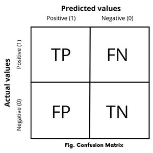
Consider a binary classification with two possible outcomes; in which the outputs are labelled either as class 1(positive) or class 0(negative).

• True Positive -* If the classifier predicts the output as 1 (positive) and the actual value is also 1(positive) then it is called True Positive(TP).*

• **False Negative **- If the classifier predicts the output as 0(negative) but in real actual value is 1(positive) then it is called False Negative(FN).

• True Negative - if the classifier predicts the output as 0(negative) and the actual value is also 0(negative) then it is called True Negative(TN).

• False Positive -* if the classifier predicts the output as 1(positive) but the actual value is 0(negative) then it is called False Positive(FP).*

The confusion matrix allows more detailed error analysis and is not limited to binary classification. A confusion matrix can be used for multi-class classifiers as well.

Using these values, you can compute other metrics that will help you to understand model performance more accurately.

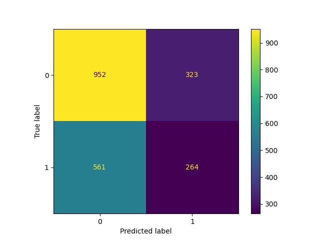
## Confusion matrix
from sklearn.metrics import confusion_matrix
from sklearn.metrics import ConfusionMatrixDisplay
cm = confusion_matrix(y_test, y_predicts)
disp = ConfusionMatrixDisplay(confusion_matrix=cm, 
                              display_labels=clf.classes_)
disp.plot()
plt.show()

2. Accuracy

Accuracy measures the fraction of total observations that are correctly classified. It is a ratio of the number of total correct classifications to the total number of observations.

Accuracy=Total,correct,predictionsTotal,number,of,observation Accuracy=TP+TNTP+FP+TN+FN

Accuracy metrics might not be a good choice to evaluate imbalanced data. Because it is easy to get high accuracy score by simply classifying all observations as the majority class. Consider an example, where data contain 95 positive observations and only 5 negative observations, then in this case classifying all values as positive, would give you a 0.95 accuracy score.

## Accuracy score.
from sklearn.metrics import accuracy_score
accuracy = accuracy_score(y_test, y_predict)
print("Accuracy Score: %.3f" %(accuracy))

Accuracy Score: 0.579

3. Precision

Precision measures the accuracy of the positive prediction i.e. it measures the ratio of positive class out of the total predicted positively by a classifier. Precision helps you to answer the question "How precisely a classifier will predict the positive class?"

Precision is the number of true positive results divided by the number of all positive results, including those that are not identified correctly.

$$Precision = \frac{TP}{TP + FP}$$

• TP is the number of true positives.

• FP is the number of false positives.

Precision measures the quality of an algorithm. Higher precision means that the algorithm returns more relevant results than irrelevant ones.

For example: Consider a brain surgeon removing cancerous cells from a patient's brain. A surgeon should remove all cancerous cells since any remaining cancer cells will regenerate. Conversely, the surgeon must not remove healthy brain cells. In this case, higher precision ensures that the surgeon removes only cancer cells. Greater precision decreases the chances of removing healthy cells while lowering the chances of removing all cancer cells.

The higher value for perfect precision is 1.0, which means that all results are relevant(True Positive) when the algorithm does not predict any false positive(FP=0), which is practically impossible.

# precision score
from sklearn.metrics import precision_score
precision = precision_score(y_test, y_predict)
print("Precision Score: %.3f" %(precision))

Precision Score: 0.450

A precision score would be more useful when you want the classifier not to label as positive a sample that is negative.

4. Recall or Sensitivity (True Positive Rate)

It measures the ratio of positive instances that are correctly detected by the classifier. Recall helps you to answer the question "What proportion of actual positives is correctly classified?"

Recall is the number of true positive results divided by the number of all samples that should have been identified as positive.

$$Recall = \frac{TP}{TP + FN}$$

• FN is the number of false negatives.

We can say that recall is the measure of quantity. A higher recall means that an algorithm returns most of the relevant results whether or not irrelevant ones are also returned. Considering the above removing cancerous cells from a patient's brain example, here the higher recall ensures that the surgeon has removed all cancer cells. but as higher recall increases the chances of removing all the cancerous cells, also increases the chances of removing healthy cells.

The higher value for the perfect recall is 1.0, which means that all results are relevant(True Positive) when the algorithm does not predict any false negative(FN=0).

# recall score
from sklearn.metrics import recall_score
recall = recall_score(y_test, y_predict)
print("Recall Score: %.3f" %(recall))

Recall Score: 0.320

F1 Score

The model with higher recall and higher precision would be the perfect classifier but an increase in the recall will decrease the precision value and vice-versa. So, we can evaluate the model performance with a single measure using precision and recall and it is called f1-score.

F1-score is a metric to evaluate the binary classification based on a prediction of the positive class. It measures the test accuracy. F1-score is the harmonic mean of the precision and recall represented by the following formula.

$$F1_{score} = 2 \* \frac{precision * recall}{precision + recall}$$

The highest possible value of an F-score is 1.0 indicating perfect precision and recall and the lowest possible value is 0. if either precision or recall is zero. The higher the F-score better the model performance.

# f1-score
from sklearn.metrics import f1_score
score = f1_score(y_test, y_predict, average='macro')
print("F1 Score: %.3f" %(score))

F1 Score: 0.528

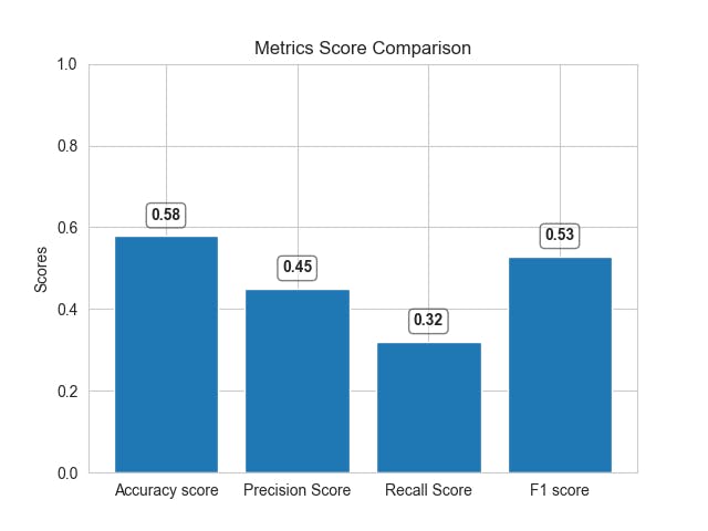
We can see that, there is a difference between scores by different metrics. The accuracy might seem high but does not consider the distribution of data and the model is actually unable to predict correctly. Here, the f1 score will provide better model performance since it takes a distribution of data into account.

6. ROC Curve

ROC(Receiver operating characteristic curve) is another way to illustrate the model performance graphically. The ROC curve is created by plotting the true positive rate(TPR) against the false positive rate(FPR) at various thresholds.

• True Positive Rate (TPR) (Recall or Sensitivity)  - It is the ratio of the number of true positive results divided by the number of all samples that should have been identified as positive.

$$TPR = \frac{TP}{TP + FN}$$

• False Positive Rate (FPR) - It is the ratio of the number of false positive results divided by the number of all samples that should have been identified as negative(Total number of actual negatives.)

$$FPR = \frac{FP}{FP + TN}$$

It is a trade-off between TPR and FPR, so Higher TPR and lower FPR are better and the curves at the top-left side are better.

# ROC Curve
from sklearn.metrics import RocCurveDisplay
RocCurveDisplay.from_estimator(clf, X, y)
plt.plot([0, 1], linestyle="--", color='black')
plt.show()

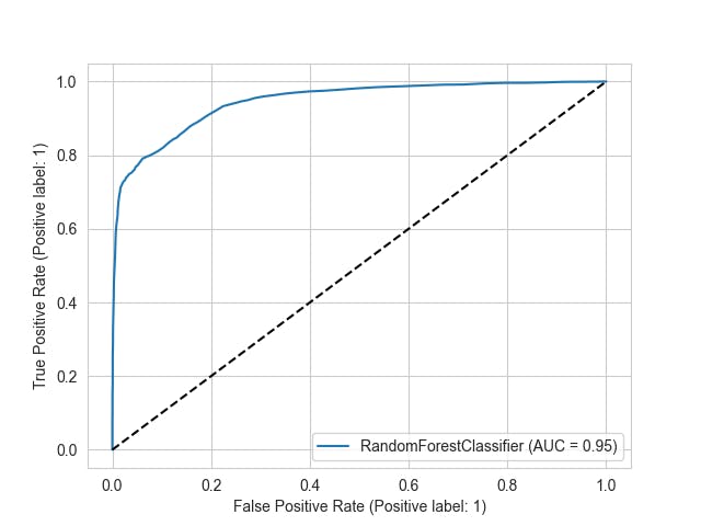
ROC curve determines the accuracy of a classifier using the area under the curve, the higher the area under the curve better the performance. In this plot, the blue line represents the ROC curve and the dashed black line represents the ROC curve at the 0.5 thresholds, where specificity = sensitivity.

Conclusion

These are some of the metrics that are commonly used for the evaluation of a classifier. As I said before, the selection of good metrics is as important as the selection of a classifier and it always depends on the data and problem that you are trying to solve.

Accuracy is often used when the classes are balanced and there is no drawback to predicting false negatives. While the f1 score is used for imbalanced class distribution and when there is a drawback to predicting false negative.

For example: Predicting someone that does not have cancer while actually, they have. In this case, the f1 score will be low since it will penalize the model more with more false negatives as compared to the accuracy.

I hope you now understand the different classification metrics for model evaluation and when to use them.

Thank you for reading.