In machine learning, decision trees are widely used supervised algorithms for both classification and regression problems. They help in finding the relationship among data points in a dataset by constructing tree structures. These tree-like structures provide an effective method of making decisions as they lay out the problem and all possible outcomes.

Decision trees are called White Box Model since it is one of the easiest algorithms to interpret and enables developers to analyze the possible consequences of a decision as it provides simple rules of classification that even be applied manually if need be. Decision trees are used in various fields such as finance, healthcare, marketing or retail, etc.

If you are interested in learning how to use decision trees in machine learning, you have come to the right place. In this blog post, I will explain what decision trees are, how they work, and what are their advantages and disadvantages with their regularization parameters to avoid the complexity of decision trees.

How do decision trees work?

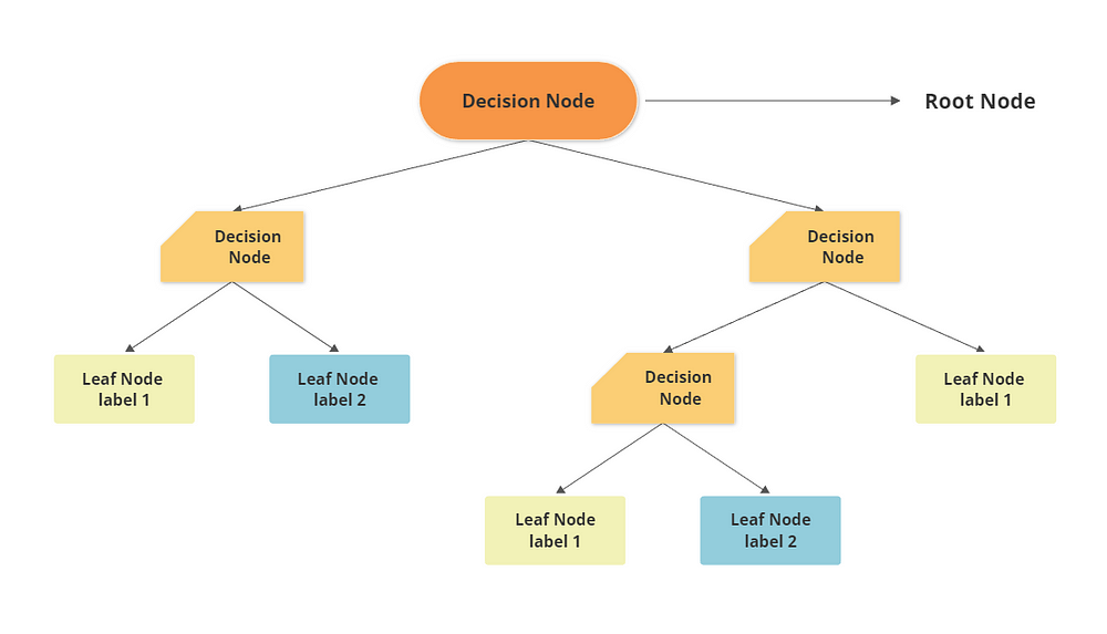
The root is the starting point of the tree, like an upside-down tree. The top root nodes split into two or more decision nodes based on the if/else conditions which further splits into more decision nodes and this process repeats until the tree reaches the bottom leaf nodes. The leaf nodes are the points where we assign a class label (for classification) or a numerical value (for regression) to the data.

The root node is, where we have the entire data set. The internal nodes are the points where we test an attribute (or a feature) of the data and split it into two or more branches based on some rule.

The main idea behind decision trees is to divide the data into smaller and more homogeneous subsets based on some criteria while preserving the relationship between the predictor variables and the response variable. This process is called recursive partitioning, and it is repeated until we reach some stopping condition, such as:

• All the data points in a subset belong to the same class (for classification) or have similar values (for regression) which are also known as a pure nodes.

• The subset is too small or too large to be further split.

• The splitting does not improve the quality of the predictions.

To build a decision tree, we need to answer two questions:

• How to choose the best attribute or feature and what should be the rule(question) to split the data at each node?

• How to measure the quality of a split?

There are different methods and metrics to answer these questions, depending on the type and objective of the problem. Some of the most common ones are:

• Information gain and entropy: These are measures of how much information or uncertainty is reduced by splitting the data based on an attribute. The higher the information gain, the better the split. Entropy is a measure of how much disorder or randomness is in the data. The lower the entropy, the more homogeneous the data.

• Gini index: This is a measure of how much impurity or diversity is in the data. The lower the Gini index, the more homogeneous the data.

• Mean squared error (MSE) and mean absolute error (MAE): These are measures of how much error or deviation is in the predictions compared to the actual values. The lower the MSE or MAE, the better the predictions.

To choose the best attribute and rule to split the data at each node, we compare different attributes and rules based on their metrics and select the one that maximizes information gain or minimizes entropy, Gini index for classification and MSE, or MAE for regression.

A prediction on new data points is made by traversing the decision tree from the root and going left or right, based on whether conditions are fulfilled or not, and finding the leaf node the new data point falls into. For classification, the output for the new data point is labeled belong to the leaf node while for regression, the output is the average of the target value of the training points in that leaf node.

The complexity of decision trees

Building a tree as described above and continuing until all leaves are pure leads to a model that is very complex and highly overfit to the training data.

The pure leaves mean that a tree is 100% accurate on the training set; each data point in the training set is in a leaf and has the correct class label.

Decision Trees often have orthogonal (perpendicular to an axis) decision boundaries (a line that separates two or more class labels), which make the model very sensitive to the small variation in training data.

In such an overfitting model, the decision boundary is too complex and fits the training data too well. This can lead to poor generalization performance on new data.

There are some techniques that can be applied to prevent overfitting, such as:

• Pre-pruning: This is a process of stopping the creation of the tree early.

• Pruning: This is a process of reducing the size and complexity of the tree by removing nodes that do not contribute much to the predictions or increase the error.

• Ensemble methods: These are methods that combine multiple decision trees to create a more robust and accurate model. Some examples are random forests and gradient boosting.

Classification And Regression Tree Algorithm

There are different types of algorithms that we can use to build a decision tree. We generally build a machine learning model using scikit-learn’s DecisionTreeClassifier class for classification and DecisionTreeRegressor class for regression.

The Scikit-learn library uses the CART(Classification And Regression Tree) algorithm for binary trees (binary classification) and Other algorithms such as the ID3 algorithm for more than two classes (multi-class classification). So let’s learn more about the CART algorithm.

The CART algorithm uses the same logic of splitting a tree as we discussed before. The algorithm splits the training set into two subsets using a single feature and a threshold value.

A selection of features and threshold is done by using Information gain, Entropy, or Gini Index. It searches for the pair(feature, threshold/condition) that produces the purest subsets by minimizing the cost function. The selection of purest subsets continues recursively until it reaches maximum depth.

The CART algorithm is also known as the greedy algorithm since it greedily searches for an optimum split at the top level (to find the root node with minimum impurity) and then repeats the process at each level.

It does not check whether or not the split will lead to the lowest possible impurity several levels down. This often produces a good solution but it is not certain to be the optimal solution. The algorithm with an optimal solution can lead to higher computational complexity for training datasets and that is why we must select a reasonably good solution.

Regularization

Decision trees make very few assumptions about the training data unlike linear models (which assume data must be linear for example). The decision trees are often called a nonparametric model because the number of parameters is not determined before training.

The predictions in the decision tree do not depend on the predetermined number of parameters such as in parametric models like linear models, where a degree of freedom is limited which reduced the risk of overfitting (but increases the risk of underfitting).

The deeper the decision tree, the more complex and fitter the model, but it often leads to overfitting

In the decision tree, prediction depends on the data if the dataset consists of noise or random fluctuations in training data. Then the model with higher complexity overfits the training data, which will memorize the data instead of learning desired patterns. As a result, it performs well on training data but does not generalize on unseen data since those concepts do not apply to the new unseen data. Because of the overfitting, the model becomes too sensitive to small variations in the data, which results in high variance.

To overcome the problem of overfitting, we can reduce the complexity of the model by reducing the Decision Tree’s freedom(depth of the tree) during training. This is known as regularization.

The regularization hyperparameters depend on the algorithm we used, but generally, one of the causes of overfitting in the decision tree is the depth of the tree.

In Scikit-learn, this is controlled by the max_depth hyperparameter. The decision tree with a single max_depth is called a decision stump.

The Decision Tree Classifier class has a few other parameters that similarly help in reducing the shape of the Decision Tree:

• min_sample_split - Minimum number of samples a node must have before it can be split.

• min_sample_leaf - The minimum number of samples a leaf node must have

• min_weight_fraction_leaf - Same as min_sample_leaf but expressed as a fraction of the total number of weighted instances.

• max_leaf_node - Maximum number of leaf nodes.

• max_features - Maximum number of features are evaluated for splitting at each node.

Increasing min_* hyperparameters or reducing max_* hyperparameters will regularize the model.

Advantages and Disadvantages of decision trees

Decision trees have several advantages, such as:

• They are easy to understand and interpret, as they mimic human reasoning and logic.

• They can handle both categorical and numerical data without feature transformation as does not affect the performance of algorithm, as well as missing values.

• They can deal with high-dimensional data and complex relationships among features.

• They are non-parametric, meaning they do not make any assumptions about the distribution or structure of the data.

However, decision trees also have some disadvantages, such as:

• They can be prone to overfitting, meaning they can capture too much noise or variance in the data and perform poorly on new or unseen data.

• They can be unstable, meaning small changes in the data can lead to large changes in the structure and predictions of the tree.

• They can be biased, meaning they can favor certain features or classes over others due to their splitting criteria.

A decision tree is a graphical representation of a series of choices and outcomes. They are one of the most popular, simple & easy to interpret non-parametric algorithms.

However, decision trees do not generalize well when working with large datasets. It leads to high computational complexity in training data resulting in an overfitting model.

But that does not mean decision trees are not usable in production. Often the combination of multiple decision trees (random forest & xgboost algorithm) gives better performance than complex models of machine learning.

I hope this article helps you learn about the working of decision trees. In the next blog post, I will explain the practical implementation of decision trees using Python and Scikit-learn.

Thank you so much for reading.

Resources —

1. Data Science from Scratch First Principles with Python Book

2. Hands–On Machine Learning with Scikit–Learn and TensorFlow 2nd edition Book

3. Introduction to Machine Learning with Python Book

4. Decision Tree learning by wikipedia