Machine learning is a field of study that gives computers the ability to learn without being explicitly programmed. — according to Arthur Samuel (1959)

In machine learning, algorithms predict the output by learning patterns and trends in given data. The main concern in the model function is to minimize the error and make the most accurate predictions using algorithms.

Classification and Regression algorithms are supervised machine learning algorithms used for prediction in machine learning and work with labelled data. They mainly differ in how they are used for different machine learning problems. Classification algorithms are used to predict discrete values such as True or False, spam or not spam. However, Regression algorithms are used to predict continuous values such as Salary, Housing Prices, etc. Linear regression is one of the regression algorithms used to predict continuous values.

Regression Analysis

Before we study linear regression, let’s understand what regression is? Regression analysis is a statistical method to estimate the relationships between a dependent variable (Output) and one or more independent variables (inputs). It will help you to understand the association of input variables with the output variable by observing the output variable for specific changes in the input variables.

In statistics, machine learning and data science, the input variables are called Independent variables(or ‘Predictors’, ‘features’, or ‘attributes’) denoted by X and output variables are called Dependent Variables(or ‘label’, ‘response’) denoted by y.

There are various types of regressions used in Machine learning. Each regression method has its importance, but all of these regression methods use the same concepts to minimise the error by estimating the relationships between the independent and dependent variables.

In this beginner’s guide, you’ll study the linear regression algorithm of machine learning and its implementation from scratch using gradient descent and its mathematical equations to help you to understand how it works.

Linear Model Representation

Linear Regression is one of the most straightforward and classic statistical models. It assumes a linear relationship between the independent variable(X) and the single dependent variable(y). The linear relationship means that if the value of X increases, y also increases or if X decreases, y also decreases.

Linear regression made predictions by finding the relationship between the two variables by fitting a linear equation to the given data. When there is only a single input variable(X), the method is called Simple/Univariate Linear Regression. The mathematical representation of simple linear regression is as below.

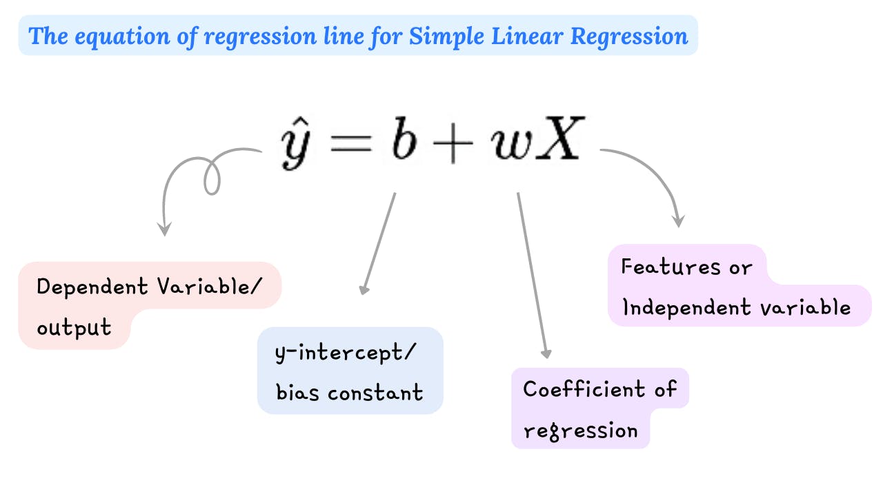
In simple linear regression, we assume that for a fixed value of X the predicted y is a linear function of X. This unknown linear function is denoted by the equation as shown above. The regression line that we fit on data is the estimated value of this linear function(y_hat).

The response(y_hat) is a weighted sum of the values of the features and a constant called the y-intercept/bias constant(b). The weighted sum means that the one scale factor (w) is assigned to each input feature(X), called the slope/ coefficient of regression.

If we plot the data points on a graph, it will be a scatter plot on the x-y plane, as shown in the above figure, and we are trying to plot the best possible straight line(regression line in the figure) that passes through these scatter data points.

Linear models find the best-fit straight line(regression line) which passes through the data points by learning parameters(intercept and coefficient of regression) by finding the relationships between these two variables.

We can say that the objective of the regression model is to find the best-fit straight line by estimating the optimum values of these parameters.

Model evaluation (Cost Function)

But how do you find the optimal values of parameters? The optimal values of parameters are those values which minimize the error between the actual data value and the value predicted by the model. To reduce error, the model could make more accurate predictions which would mean the model is closer to actual data.

To measure how accurately the linear model predicts the output. We can use the mean squared error method. Metrics used for model evaluation is a cost function or loss function.

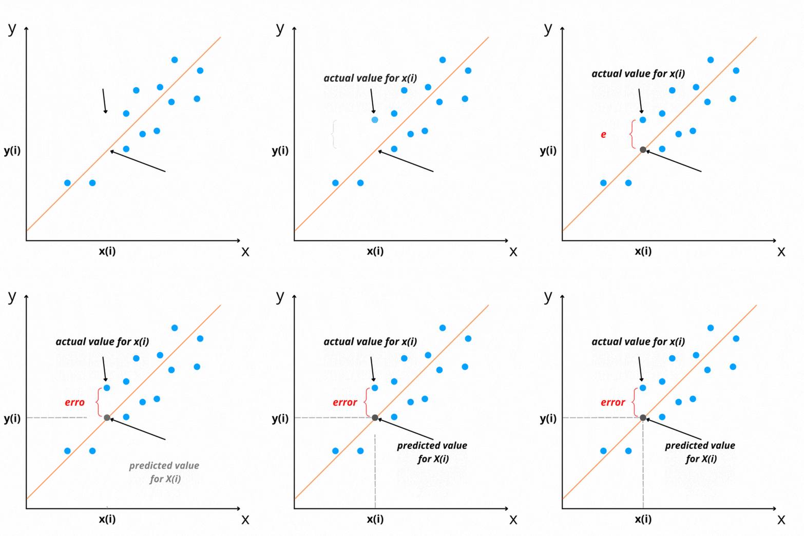
The difference between actual and predicted values is called residual(e). It can be negative or positive depending on whether the model over-predicts or under-predict value. Therefore, Calculating the total error by adding all residuals can lead to zero(assuming that line is the best-fit line).

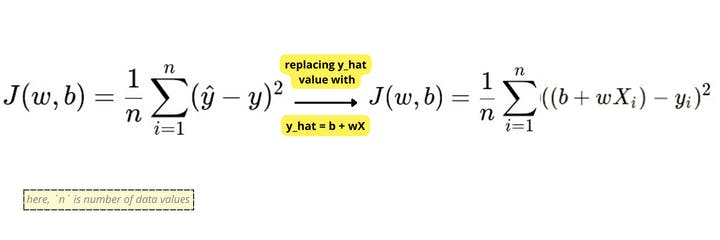
We take the sum of squares of these error terms to avoid the cancellation effect. Then we calculate the average of the sum of squares of the residuals. That is why the name Mean Squared Error(MSE).

This is an equation of cost function{J(w, b)} for simple linear regression.

Implementation of Simple Linear Regression using Gradient Descent from scratch

We will use the gradient descent method to find the most optimal values of the parameters on our cost function.

Gradient descent is an optimization algorithm that uses an iterative method to find the optimum values of parameters and to find local minimum values of the cost function. In the gradient descent, we simultaneously update the values of the w and b by computing partial derivatives with respect to w and b on the cost function until we find the minimum value of the error.

The followings are the equation of the partial derivatives on cost function with respect to w and b and the equation to update the values of w and b.

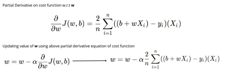
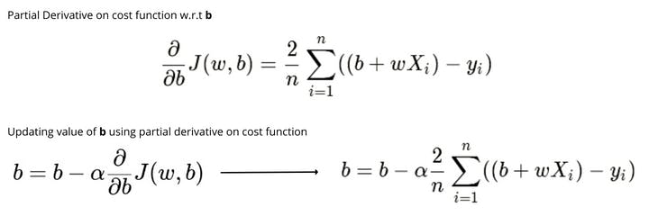
The learning rate(alpha) is one of the decisive hyperparameters in gradient descent for updating values of parameters. Since the choice of the learning rate will have a significant impact on the implementation of the gradient descent algorithm. If the learning rate is too low, then the gradient descent works, but it will take a long time to find the local minimum since it will take tiny baby steps to reach the lowest value of error. In contrast, if the learning rate is too large, the gradient descent will miss the local minimum and never find the local minimum and fail to converge.

The following code is for implementing the simple linear regression from scratch using gradient descent. I have used the dataset of housing prices with a feature size to predict the price using libraries like CSV for reading csv files, NumPy for numerical computation, and Matplotlib for plotting to scatter plots.

We first initialize the values of w and b with zero and then for each iteration we compute the error and update the values of w and b using the above equations.

Assumption of Linear Regression

There are several assumptions about the predictor variables, the response variables and their relationship. These are some common assumptions that can help to improve the performance of the linear regression model.

• As we know, linear regression assumes that the relationship between the input(X) and output(y) is linear. Before fitting a linear model on data, you should determine if there is a relationship between the two variables. You can use a scatterplot to determine the relation between two variables. Log transformation on feature data can help to make it linear.
• Linear regression assumes that the feature variables not being correlated to each other. It will overfit the data if the features are highly correlated. Consider removing highly correlated features for better model performance.
• Linear regression assumes that there are no outliers present in the variables. Consider removing outliers from both input and output variables if possible.
• Linear regression assumes that error has a constant variance(homoscedasticity). The absence of homoscedasticity is called heteroscedasticity. To check the heteroscedasticity, plot the scatter plot of the residuals versus predicted values. The heteroscedasticity leads to less accurate parameter estimations and biased standard error.
• Linear regression will predict more accurate results for Gaussian distributions. If the distribution of the input feature is not Gaussian, you can use log transformation on features to make the distribution more Gaussian.
• For better performance of linear regression, consider rescaling the features using Standardization or Normalization.

Simple linear regression is one of the methods of linear regression. This article explained the simple linear regression with its implementation. We used mathematical equations to implement the model from scratch and to understand how the model works with a brief introduction of gradient descent and the assumption of linear regression.

Thank you for reading.